Unconstrained optimization

• The rationality of the step size

In the following section, we would begin to discuss two conditions which a_k(the step size) have to satisfy. If the two conditions are both satisfied, we could say that the proper step size, from x_k to x_(k+1), has been found. The first condition called “sufficient decrease condition”.  Intuitively, this condition keeps that the value at x_(k+1) should be smaller than x_(k)`s, which is required to reach the convergence. The second one is called “curvature condition”. This condition keeps that the derivative of f at x_k must be smaller than x_(k+1)`s.

• Sufficient decrease condition

A proper a_k must satisfy sufficient decrease condition. We could make the following descriptions about this condition:

f( x_(k+1) ) <= f( x_k ) + c_1 * a_k * ▽f_k^T * p_k;

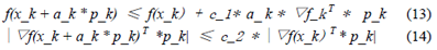
if we plugin EQ1, we have

f( x_k + a_k * p_k ) <= f( x_k ) _ c_1 * a_k * ▽f_k^T * p_k

where f( x_k ) is the value of f at x_k; ▽f_k means the gradient at x_k; p_k means the direction from x_k to x_(k+1); a_k means the step size and c_1 is a constant that belongs to [0, 1]

If p_k is the decent direction of function f, we have ▽f_k * p_k < 0. So f( x_k + 1 )<f( x_k ).

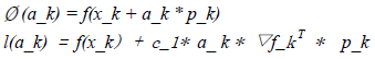
As only a_k is a variable, we could rewrite as followed:

Ø(a_k) ≤ l(a_k), where

 

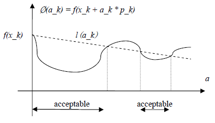
We could visualize the condition as below:

If the step size could make Ø(a_k) in the acceptable interval, the condition is satisfied.

• Curvature condition

We could describe this condition as following:

 

or     

In the above equation, ▽f_(k+1) is the gradient at x_(k+1); p_k is the decent direction and c_2 is an constant belongs to [0 1] and usually set as 0.9.

When p_k is the decent direction of the function f, then ▽f_k * p_k < 0

So, it means ▽f _k+1 ≥ c_2 * ▽f_k

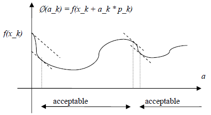
From the plot below, we could see that the equation above requires that the decent “speed” at x_(k+1)should be smaller than x_k`s.

• Wolfe condition

Wolfe condition could be seemed as the combination of the two conditions mentioned above, which means the a_k should meet the following equations.

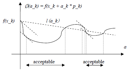
We could visualize the condition as:

In some real optimization application, we may have to use another condition, called string Wolfe condition, which is stemmed from the Wolfe condition. In this case, the a_k need to meet the followings:

The only difference between those two conditions is the strong Wolfe condition avoids the possible positive value of  ▽f(x_k + a_k * p_k).

 

To be continued.