Saturday, March 28, 2009

Eigenface, from Wiki

Eigenfaces are a set of eigenvectors used in the computer vision problem of human face recognition. The approach of using eigenfaces for recognition was developed by Sirovich and Kirby (1987) and used by Matthew Turk and Alex Pentland in face classification. It is considered the first successful example of facial recognition technology.[citation needed] These eigenvectors are derived from the covariance matrix of the probability distribution of the high-dimensional vector space of possible faces of human beings.

Eigenface generation

To generate a set of eigenfaces, a large set of digitized images of human faces, taken under the same lighting conditions, are normalized to line up the eyes and mouths. They are then all resampled at the same pixel resolution. Eigenfaces can be extracted out of the image data by means of a mathematical tool called principal component analysis (PCA).

The eigenfaces that are created will appear as light and dark areas that are arranged in a specific pattern. This pattern is how different features of a face are singled out to be evaluated and scored. There will be a pattern to evaluate symmetry, if there is any style of facial hair, where the hairline is, or evaluate the size of the nose or mouth. Other eigenfaces have patterns that are less simple to identify, and the image of the eigenface may look very little like a face.

The technique used in creating eigenfaces and using them for recognition is also used outside of facial recognition. This technique is also used for handwriting analysis, lip reading, voice recognition, sign language/hand gestures and medical imaging. Therefore, some do not use the term eigenface, but prefer to use 'eigenimage'. Research that applies similar eigen techniques to sign language images has also been made.

Informally, eigenfaces are a set of "standardized face ingredients", derived from statistical analysis of many pictures of faces. Any human face can be considered to be a combination of these standard faces. For example, your face might be composed of the average face plus 10% from eigenface 1, 55% from eigenface 2, and even -3% from eigenface 3. Remarkably, it does not take many eigenfaces summed together to give a fair likeness of most faces. Also, because a person's face is no longer recorded by a digital photograph, but instead as just a list of values (one value for each eigenface in the database used), much less space is taken for each person's face.

Practical implementation

Here are the steps involved in creating a set of eigenfaces:

  1. Prepare a training set. The faces constituting the training set should be of prepared for processing, in the sense that they should all have the same resolution and that the faces should be roughly aligned. Each image is seen as one vector, simply by concatenating the rows of pixels in the original image. A greyscale image with r rows and c columns is therefore represented as a vector with r x c elements. In the following discussion we assume all images of the training set are stored in a single matrix T, where each row of the matrix is an image.
  2. Subtract the mean. The average image a has to be calculated and subtracted from each original image in T.
  3. Calculate the eigenvectors and eigenvalues of the covariance matrix S. Each eigenvector has the same dimensionality as the original images and can itself be seen as an image. The eigenvectors of this covariance matrix are therefore called eigenfaces. They are the directions in which the images in the training set differ from the mean image. In general this will be a computationally expensive step (when it is at all possible), but the practical applicability of eigenfaces stems from the possibility to compute the eigenvectors of S efficiently, without ever computing S explicitly, as detailed below.
  4. Choose the principal components. The D x D covariance matrix will result in D eigenvectors, each representing a direction in the image space. Keep the eigenvectors with largest associated eigenvalue.

The eigenfaces can now be used to represent new faces: we can project a new (mean-subtracted) image on the eigenfaces and thereby record how that new face differs from the mean face. The eigenvalues associated with each eigenface represent how much the images in the training set vary from the mean image in that direction. We lose information by projecting the image on a subset of the eigenvectors, but we minimise this loss by keeping those eigenfaces with the largest eigenvalues. For instance, if we are working with a 100 x 100 image, then we will obtain 10,000 eigenvectors. In practical applications, most faces can typically be identified using a projection on between 100 and 150 eigenfaces, so that most of the 10,000 eigenvectors can be discarded.

Computing the eigenvectors

Performing PCA directly on the covariance matrix of the images is often computationally infeasible. If small, say 100 x 100, greyscale images are used, each image is a point in a 10,000-dimensional space and the covariance matrix S is a matrix of 10,000 x 10,000 = 108 elements. However the rank of the covariance matrix is limited by the number of training examples: if there are N training examples, there will be at most N-1 eigenvectors with non-zero eigenvalues. If the number of training examples is smaller than the dimensionality of the images, the principal components can be computed more easily as follows.

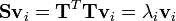
Let T be the matrix of preprocessed training examples, where each row contains one mean-subtracted image. The covariance matrix can then be computed as S = TT T and the eigenvector decomposition of S is given by

\mathbf{Sv}_i = \mathbf{T}^T\mathbf{Tv}_i = \lambda_i \mathbf{v}_i

However TTT is a large matrix, and if instead we take the eigenvalue decomposition of

\mathbf{TT}^T\mathbf{u}_i = \lambda_i \mathbf{u}_i

then we notice that by pre-multiplying both sides of the equation with TT, we obtain

\mathbf{T}^T\mathbf{TT}^T\mathbf{u}_i = \lambda_i \mathbf{T}^T\mathbf{u}_i

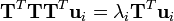
Meaning that, if ui is an eigenvector of TTT, then vi=TTui is an eigenvector of S. If we have a training set of 300 images of 100 x 100 pixels, the matrix TTT is a 300 x 300 matrix, which is much more manageable than the 10000 x 10000 covariance matrix. Notice however that the resulting vectors vi are not normalised; if normalisation is required it should be applied as an extra step.

Use in facial recognition

Facial recognition was the source of motivation behind the creation of eigenfaces. For this use, eigenfaces have advantages over other techniques available, such as the system's speed and efficiency. Using eigenfaces is very fast, and able to functionally operate on lots of faces in very little time. Unfortunately, this type of facial recognition does have a drawback to consider: trouble recognizing faces when they are viewed with different levels of light or angles. For the system to work well, the faces need to be seen from a frontal view under similar lighting. Face recognition using eigenfaces has been shown to be quite accurate. By experimenting with the system to test it under variations of certain conditions, the following correct recognitions were found: an average of 96% with light variation, 85% with orientation variation, and 64% with size variation. (Turk & Pentland 1991, p. 590)

To complement eigenfaces, another approach has been developed called eigenfeatures. This combines facial metrics (measuring distance between facial features) with the eigenface approach. Another method, which is competing with the eigenface technique uses 'fisherfaces'. This method for facial recognition is less sensitive to variation in lighting and pose of the face than the method using eigenfaces.

A more modern alternative to eigenfaces and fisherfaces is the active appearance model, which decouples the face's shape from its texture: it does an eigenface decomposition of the face after warping it to mean shape. This allows it to perform better on different projections of the face, and when the face is tilted.
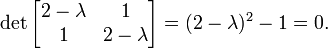
Eigenvalue, eigenvector and eigenspace

In mathematics, given a linear transformation, an eigenvector of that linear transformation is a nonzero vector which, when that transformation is applied to it, may change in length, but not direction.

For each eigenvector of a linear transformation, there is a corresponding scalar value called an eigenvalue for that vector, which determines the amount the eigenvector is scaled under the linear transformation. For example, an eigenvalue of +2 means that the eigenvector is doubled in length and points in the same direction. An eigenvalue of +1 means that the eigenvector is unchanged, while an eigenvalue of −1 means that the eigenvector is reversed in sense. An eigenspace of a given transformation for a particular eigenvalue is the set (linear span) of the eigenvectors associated to this eigenvalue, together with the zero vector (which has no direction).

In linear algebra, every linear transformation between finite-dimensional vector spaces can be expressed as a matrix, which is a rectangular array of numbers arranged in rows and columns. Standard methods for finding eigenvalues, eigenvectors, and eigenspaces of a given matrix are discussed below.

These concepts play a major role in several branches of both pure and applied mathematics—appearing prominently in linear algebra, functional analysis, and to a lesser extent in nonlinear mathematics.

Many kinds of mathematical objects can be treated as vectors: functions, harmonic modes, quantum states, and frequencies, for example. In these cases, the concept of direction loses its ordinary meaning, and is given an abstract definition. Even so, if this abstract direction is unchanged by a given linear transformation, the prefix "eigen" is used, as in eigenfunction, eigenmode, eigenstate, and eigenfrequency.

Definitions

Linear transformations of a vector space, such as rotation, reflection, stretching, compression, shear or any combination of these, may be visualized by the effect they produce on vectors. In other words, they are vector functions. More formally, in a vector space L, a vector function A is defined if for each vector x of L there corresponds a unique vector y = A(x) of L. For the sake of brevity, the parentheses around the vector on which the transformation is acting are often omitted. A vector function A is linear if it has the following two properties:

where x and y are any two vectors of the vector space L and α is any scalar.[13] Such a function is variously called a linear transformation, linear operator, or linear endomorphism on the space L.

Given a linear transformation A, a non-zero vector x is defined to be an eigenvector of the transformation if it satisfies the eigenvalue equation Ax = λx for some scalar λ. In this situation, the scalar λ is called an eigenvalue of A corresponding to the eigenvector x.[14]

The key equation in this definition is the eigenvalue equation, Ax = λx. That is to say that the vector x has the property that its direction is not changed by the transformation A, but that it is only scaled by a factor of λ. Most vectors x will not satisfy such an equation: a typical vector x changes direction when acted on by A, so that Ax is not a multiple of x. This means that only certain special vectors x are eigenvectors, and only certain special numbers λ are eigenvalues. Of course, if A is a multiple of the identity matrix, then no vector changes direction, and all non-zero vectors are eigenvectors.

The requirement that the eigenvector be non-zero is imposed because the equation A0 = λ0 holds for every A and every λ. Since the equation is always trivially true, it is not an interesting case. In contrast, an eigenvalue can be zero in a nontrivial way. Each eigenvector is associated with a specific eigenvalue. One eigenvalue can be associated with several or even with an infinite number of eigenvectors.

Fig. 2. A acts to stretch the vector x, not change its direction, so x is an eigenvector of A.

Geometrically (Fig. 2), the eigenvalue equation means that under the transformation A eigenvectors experience only changes in magnitude and sign—the direction of Ax is the same as that of x. The eigenvalue λ is simply the amount of "stretch" or "shrink" to which a vector is subjected when transformed by A. If λ = 1, the vector remains unchanged (unaffected by the transformation). A transformation I under which a vector x remains unchanged, Ix = x, is defined as identity transformation. If λ = −1, the vector flips to the opposite direction; this is defined as reflection.

If x is an eigenvector of the linear transformation A with eigenvalue λ, then any scalar multiple αx is also an eigenvector of A with the same eigenvalue. Similarly if more than one eigenvector share the same eigenvalue λ, any linear combination of these eigenvectors will itself be an eigenvector with eigenvalue λ. [15]. Together with the zero vector, the eigenvectors of A with the same eigenvalue form a linear subspace of the vector space called an eigenspace.

The eigenvectors corresponding to different eigenvalues are linearly independent[16] meaning, in particular, that in an n-dimensional space the linear transformation A cannot have more than n eigenvectors with different eigenvalues.[17]

If a basis is defined in vector space, all vectors can be expressed in terms of components. For finite dimensional vector spaces with dimension n, linear transformations can be represented with n × n square matrices. Conversely, every such square matrix corresponds to a linear transformation for a given basis. Thus, in a two-dimensional vector space R2 fitted with standard basis, the eigenvector equation for a linear transformation A can be written in the following matrix representation:

 \begin{bmatrix} a_{11} & a_{12} \\ a_{21} & a_{22} \end{bmatrix} \begin{bmatrix} x \\ y \end{bmatrix} = \lambda \begin{bmatrix} x \\ y \end{bmatrix},

where the juxtaposition of matrices denotes matrix multiplication.

Left and right eigenvectors

The word eigenvector formally refers to the right eigenvector xR. It is defined by the above eigenvalue equation AxR = λRxR, and is the most commonly used eigenvector. However, the left eigenvector xL exists as well, and is defined by xLA = λLxL.

Characteristic equation

When a transformation is represented by a square matrix A, the eigenvalue equation can be expressed as

A \mathbf{x} - \lambda I \mathbf{x} = \mathbf{0}.

This can be rearranged to

(A - \lambda I) \mathbf{x} = \mathbf{0}.

If there exists an inverse

(A - \lambda I)^\mathbf{-1},

then both sides can be left multiplied by the inverse to obtain the trivial solution: x = 0. Thus we require there to be no inverse by assuming from linear algebra that the determinant equals zero:

\det(A - \lambda I) = \mathbf{0}.

The determinant requirement is called the characteristic equation (less often, secular equation) of A, and the left-hand side is called the characteristic polynomial. When expanded, this gives a polynomial equation for λ. The eigenvector x or its components are not present in the characteristic equation.

Example

The matrix

\begin{bmatrix} 2  & 1\\1 & 2 \end{bmatrix}

defines a linear transformation of the real plane. The eigenvalues of this transformation are given by the characteristic equation

\det\begin{bmatrix} 2-\lambda  & 1\\1 & 2-\lambda \end{bmatrix} = (2-\lambda)^2 - 1 = 0.

The roots of this equation (i.e. the values of λ for which the equation holds) are λ = 1 and λ = 3. Having found the eigenvalues, it is possible to find the eigenvectors. Considering first the eigenvalue λ = 3, we have

\begin{bmatrix} 2  & 1\\1 & 2 \end{bmatrix}\begin{bmatrix}x\\y\end{bmatrix} = 3 \begin{bmatrix}x\\y\end{bmatrix}.

After matrix-multiplication \begin{bmatrix} 2x+y  \\x+2y \end{bmatrix} = 3 \begin{bmatrix}x\\y\end{bmatrix}.

This matrix equation represents a system of two linear equations 2x + y = 3x and x + 2y = 3y. Both the equations reduce to the single linear equation x = y. To find an eigenvector, we are free to choose any value for x, so by picking x=1 and setting y=x, we find the eigenvector to be

\begin{bmatrix}1\\1\end{bmatrix}.

We can check this is an eigenvector by checking that :\begin{bmatrix}2&1\\1&2\end{bmatrix}\begin{bmatrix}1\\1\end{bmatrix} = \begin{bmatrix}3\\3\end{bmatrix}. For the eigenvalue λ = 1, a similar process leads to the equation x = − y, and hence the eigenvector is given by

\begin{bmatrix}1\\-1\end{bmatrix}.

The complexity of the problem for finding roots/eigenvalues of the characteristic polynomial increases rapidly with increasing the degree of the polynomial (the dimension of the vector space). There are exact solutions for dimensions below 5, but for dimensions greater than or equal to 5 there are generally no exact solutions and one has to resort to numerical methods to find them approximately. For large symmetric sparse matrices, Lanczos algorithm is used to compute eigenvalues and eigenvectors.

Eigenfaces

Fig. 9. Eigenfaces as examples of eigenvectors

In image processing, processed images of faces can be seen as vectors whose components are the brightnesses of each pixel.[24] The dimension of this vector space is the number of pixels. The eigenvectors of the covariance matrix associated to a large set of normalized pictures of faces are called eigenfaces; this is an example of principal components analysis. They are very useful for expressing any face image as a linear combination of some of them. In the facial recognition branch of biometrics, eigenfaces provide a means of applying data compression to faces for identification purposes. Research related to eigen vision systems determining hand gestures has also been made.

Similar to this concept, eigenvoices represent the general direction of variability in human pronunciations of a particular utterance, such as a word in a language. Based on a linear combination of such eigenvoices, a new voice pronunciation of the word can be constructed. These concepts have been found useful in automatic speech recognition systems, for speaker adaptation.

Wednesday, March 25, 2009

Difference of Gaussians(Wiki)

Difference of Gaussians

In computer vision, Difference of Gaussians is a grayscale image enhancement algorithm that involves the subtraction of one blurred version of an original grayscale image from another, less blurred version of the original. The blurred images are obtained by convolving the original grayscale image with Gaussian kernels having differing standard deviations. Blurring an image using a Gaussian kernel suppresses only high-frequency spatial information. Subtracting one image from the other preserves spatial information that lies between the range of frequencies that are preserved in the two blurred images. Thus, the difference of Gaussians is equivalent to a band-pass filter that discards all but a handful of spatial frequencies that are present in the original grayscale image.[1]

Mathematics of Difference of Gaussians

The Difference of Gaussians (DOG) is a wavelet mother function of null total sum which approximates the Mexican Hat wavelet by subtracting a wide Gaussian from a narrow Gaussian, as defined by this formula in one dimension:


f(x;\mu,\sigma_1,\sigma_2)
=
\frac{1}{\sigma_1\sqrt{2\pi}} \, \exp \left( -\frac{(x- \mu)^2}{2\sigma_1^2} \right)-\frac{1}{\sigma_2\sqrt{2\pi}} \, \exp \left( -\frac{(x- \mu)^2}{2\sigma_2^2} \right).

and for the centered two-dimensional case (see Gaussian blur):


f(u,v,\sigma)
=
\frac{1}{2\pi \sigma^2} \exp ^{-(u^2 + v^2)/(2 \sigma^2)} - \frac{1}{2\pi K^2 \sigma^2}  \exp ^{-(u^2 + v^2)/(2 K^2 \sigma^2)}

Details and applications

As an image enhancement algorithm, the Difference of Gaussians can be utilized to increase the visibility of edges and other detail present in a digital image. A wide variety of alternative edge sharpening filters operate by enhancing high frequency detail, but because random noise also has a high spatial frequency, many of these sharpening filters tend to enhance noise, which can be an undesirable artifact. The Difference of Gaussians algorithm removes high frequency detail that often includes random noise, rendering this approach one of the most suitable for processing images with a high degree of noise. A major drawback to application of the algorithm is an inherent reduction in overall image contrast produced by the operation.[1]

When utilized for image enhancement, the Difference of Gaussians algorithm is typically applied when the size ratio of kernel (2) to kernel (1) is 4:1 or 5:1. In the example images to the right, the sizes of the Gaussian kernels employed to smooth the sample image were 10 pixels and 5 pixels. The algorithm can also be used to obtain an approximation of the Laplacian of Gaussian when the ratio of size 2 to size 1 is roughly equal to 1.6[2]. The Laplacian of Gaussian is useful for detecting edges that appear at various image scales or degrees of image focus. The exact values of sizes of the two kernels that are used to approximate the Laplacian of Gaussian will determine the scale of the difference image, which may appear blurry as a result.

Differences of Gaussians have also been used for blob detection in the scale-invariant feature transform. In fact, the DOG as the difference of two Multivariate normal distribution has always a total null sum and convolving it with a uniform signal generates no response. It approximates well a second derivate of Gaussian (Laplacian of Gaussian) with K~1.6 and the receptive fields of ganglion cells in the retina with K~5. It may easily be used in recursive schemes and is used as an operator in real-time algorithms for blob detection and automatic scale selection.

Tuesday, March 24, 2009

repmat() of matlab

repmat - Replicate and tile array

Syntax

B = repmat(A,m,n)
B = repmat(A,[m n])
B = repmat(A,[m n p...])

Description

B = repmat(A,m,n) creates a large matrix B consisting of an m-by-n tiling of copies of A. The size of B is [size(A,1)*m, (size(A,2)*n]. The statement repmat(A,n) creates an n-by-n tiling.

B = repmat(A,[m n]) accomplishes the same result as repmat(A,m,n).

B = repmat(A,[m n p...]) produces a multidimensional array B composed of copies of A. The size of B is [size(A,1)*m, size(A,2)*n, size(A,3)*p, ...].

Remarks

repmat(A,m,n), when A is a scalar, produces an m-by-n matrix filled with A's value and having A's class. For certain values, you can achieve the same results using other functions, as shown by the following examples:

  • repmat(NaN,m,n) returns the same result as NaN(m,n).

  • repmat(single(inf),m,n) is the same as inf(m,n,'single').

  • repmat(int8(0),m,n) is the same as zeros(m,n,'int8').

  • repmat(uint32(1),m,n) is the same as ones(m,n,'uint32').

  • repmat(eps,m,n) is the same as eps(ones(m,n)).

Examples

In this example, repmat replicates 12 copies of the second-order identity matrix, resulting in a "checkerboard" pattern.

B = repmat(eye(2),3,4)&eye() creats an identity matrix  B =      
1     0     1     0     1     0     1     0      0     1     0     1     0     1     0     1      1     0     1     0     1     0     1     0      0     1     0     1     0     1     0     1      1     0     1     0     1     0     1     0      0     1     0     1     0     1     0     1 

The statement N = repmat(NaN,[2 3]) creates a 2-by-3 matrix of NaNs.

NOTE: Obtain from Matlab official website

Solid Angle

Solid Angle

The solid angle Omega subtended by a surface S is defined as the surface area Omega of a unit sphere covered by the surface's projection onto the sphere. This can be written as

 Omega=intint_S(n^^・da)/(r^2),

where n^^ is a unit vector from the origin, da is the differential area of a surface patch, and r is the distance from the origin to the patch. Written in spherical coordinates with phi the colatitude (polar angle) and theta for the longitude (azimuth), this becomes

 Omega=intint_Ssinphidthetadphi.

Solid angle is measured in steradians, and the solid angle corresponding to all of space being subtended is 4pi steradians.

SolidAngleCube

To see how the solid angle of simple geometric shapes can be computed explicitly, consider the solid angle Omega_(cube side) subtended by one face of a cube of side length 2a centered at the origin. Since the cube is symmetrical and has six sides, one side obviously subtends 4pi/6= steradians. To compute this explicitly, rewrite (1) in Cartesian coordinates using

n^^・da=cosphidxdy
r^2=x^2+y^2+z^2

and

cosphi=z/r
=z/(sqrt(x^2+y^2+z^2)).

Considering the top face of the cube, which is located at z= and has sides parallel the x- and y-axes,

Omega_(cube side)=int_(-a)^aint_(-a)^a(adxdy)/((x^2+y^2+a^2)^(3/2))
=2/3pi,

as expected.

SolidAngleTetrahedron

Similarly, consider a tetrahedron with side lengths a with origin at the centroid, base at z= (where r is the centroid), and bottom vertices at (-d,+/-a/2,-r) and (x_0,0,-r), where

x_0=1/3sqrt(3)a
r=1/(12)sqrt(6)a
d=1/6sqrt(3)a.

Then x runs from -d to x_0, and for the half of the base in the positive y half-plane, y can be taken to run from 0 to a/2-(a/2)/(d+x_0)(x+d)=, giving

Omega=2int_(-d)^(x_0)int_0^(1/3-x/sqrt(3))(rdydx)/((x^2+y^2+r^2)^(3/2))
=pi,

i.e., 4pi/4, as expected.

NOTE: obtained from http://mathworld.wolfram.com/SolidAngle.html