Eigenvalue, eigenvector and eigenspace

In mathematics, given a linear transformation, an eigenvector of that linear transformation is a nonzero vector which, when that transformation is applied to it, may change in length, but not direction.

For each eigenvector of a linear transformation, there is a corresponding scalar value called an eigenvalue (info) for that vector, which determines the amount the eigenvector is scaled under the linear transformation. For example, an eigenvalue of +2 means that the eigenvector is doubled in length and points in the same direction. An eigenvalue of +1 means that the eigenvector is unchanged, while an eigenvalue of −1 means that the eigenvector is reversed in sense. An eigenspace of a given transformation for a particular eigenvalue is the set (linear span) of the eigenvectors associated to this eigenvalue, together with the zero vector (which has no direction).

In linear algebra, every linear transformation between finite-dimensional vector spaces can be expressed as a matrix, which is a rectangular array of numbers arranged in rows and columns. Standard methods for finding eigenvalues, eigenvectors, and eigenspaces of a given matrix are discussed below.

These concepts play a major role in several branches of both pure and applied mathematics—appearing prominently in linear algebra, functional analysis, and to a lesser extent in nonlinear mathematics.

Many kinds of mathematical objects can be treated as vectors: functions, harmonic modes, quantum states, and frequencies, for example. In these cases, the concept of direction loses its ordinary meaning, and is given an abstract definition. Even so, if this abstract direction is unchanged by a given linear transformation, the prefix "eigen" is used, as in eigenfunction, eigenmode, eigenstate, and eigenfrequency.

Definitions

See also: Eigenplane

Linear transformations of a vector space, such as rotation, reflection, stretching, compression, shear or any combination of these, may be visualized by the effect they produce on vectors. In other words, they are vector functions. More formally, in a vector space L, a vector function A is defined if for each vector x of L there corresponds a unique vector y = A(x) of L. For the sake of brevity, the parentheses around the vector on which the transformation is acting are often omitted. A vector function A is linear if it has the following two properties:

• Additivity: A(x + y) = Ax + Ay
• Homogeneity: A(αx) = αAx

where x and y are any two vectors of the vector space L and α is any scalar.^[13] Such a function is variously called a linear transformation, linear operator, or linear endomorphism on the space L.

Given a linear transformation A, a non-zero vector x is defined to be an eigenvector of the transformation if it satisfies the eigenvalue equation Ax = λx for some scalar λ. In this situation, the scalar λ is called an eigenvalue of A corresponding to the eigenvector x.[14]

The key equation in this definition is the eigenvalue equation, Ax = λx. That is to say that the vector x has the property that its direction is not changed by the transformation A, but that it is only scaled by a factor of λ. Most vectors x will not satisfy such an equation: a typical vector x changes direction when acted on by A, so that Ax is not a multiple of x. This means that only certain special vectors x are eigenvectors, and only certain special numbers λ are eigenvalues. Of course, if A is a multiple of the identity matrix, then no vector changes direction, and all non-zero vectors are eigenvectors.

The requirement that the eigenvector be non-zero is imposed because the equation A0 = λ0 holds for every A and every λ. Since the equation is always trivially true, it is not an interesting case. In contrast, an eigenvalue can be zero in a nontrivial way. Each eigenvector is associated with a specific eigenvalue. One eigenvalue can be associated with several or even with an infinite number of eigenvectors.

Fig. 2. A acts to stretch the vector x, not change its direction, so x is an eigenvector of A.

Geometrically (Fig. 2), the eigenvalue equation means that under the transformation A eigenvectors experience only changes in magnitude and sign—the direction of Ax is the same as that of x. The eigenvalue λ is simply the amount of "stretch" or "shrink" to which a vector is subjected when transformed by A. If λ = 1, the vector remains unchanged (unaffected by the transformation). A transformation I under which a vector x remains unchanged, Ix = x, is defined as identity transformation. If λ = −1, the vector flips to the opposite direction; this is defined as reflection.

If x is an eigenvector of the linear transformation A with eigenvalue λ, then any scalar multiple αx is also an eigenvector of A with the same eigenvalue. Similarly if more than one eigenvector share the same eigenvalue λ, any linear combination of these eigenvectors will itself be an eigenvector with eigenvalue λ. ^[15]. Together with the zero vector, the eigenvectors of A with the same eigenvalue form a linear subspace of the vector space called an eigenspace.

The eigenvectors corresponding to different eigenvalues are linearly independent^[16] meaning, in particular, that in an n-dimensional space the linear transformation A cannot have more than n eigenvectors with different eigenvalues.^[17]

If a basis is defined in vector space, all vectors can be expressed in terms of components. For finite dimensional vector spaces with dimension n, linear transformations can be represented with n × n square matrices. Conversely, every such square matrix corresponds to a linear transformation for a given basis. Thus, in a two-dimensional vector space R² fitted with standard basis, the eigenvector equation for a linear transformation A can be written in the following matrix representation:

where the juxtaposition of matrices denotes matrix multiplication.

Left and right eigenvectors

The word eigenvector formally refers to the right eigenvector x_R. It is defined by the above eigenvalue equation Ax_R = λ_Rx_R, and is the most commonly used eigenvector. However, the left eigenvector x_L exists as well, and is defined by x_LA = λ_Lx_L.

Characteristic equation

Main article: Characteristic polynomial

When a transformation is represented by a square matrix A, the eigenvalue equation can be expressed as

This can be rearranged to

If there exists an inverse

then both sides can be left multiplied by the inverse to obtain the trivial solution: x = 0. Thus we require there to be no inverse by assuming from linear algebra that the determinant equals zero:

The determinant requirement is called the characteristic equation (less often, secular equation) of A, and the left-hand side is called the characteristic polynomial. When expanded, this gives a polynomial equation for λ. The eigenvector x or its components are not present in the characteristic equation.

Example

The matrix

defines a linear transformation of the real plane. The eigenvalues of this transformation are given by the characteristic equation

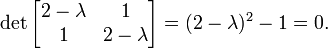
The roots of this equation (i.e. the values of λ for which the equation holds) are λ = 1 and λ = 3. Having found the eigenvalues, it is possible to find the eigenvectors. Considering first the eigenvalue λ = 3, we have

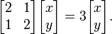
After matrix-multiplication

This matrix equation represents a system of two linear equations 2x + y = 3x and x + 2y = 3y. Both the equations reduce to the single linear equation x = y. To find an eigenvector, we are free to choose any value for x, so by picking x=1 and setting y=x, we find the eigenvector to be

We can check this is an eigenvector by checking that :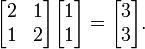 For the eigenvalue λ = 1, a similar process leads to the equation x = − y, and hence the eigenvector is given by

The complexity of the problem for finding roots/eigenvalues of the characteristic polynomial increases rapidly with increasing the degree of the polynomial (the dimension of the vector space). There are exact solutions for dimensions below 5, but for dimensions greater than or equal to 5 there are generally no exact solutions and one has to resort to numerical methods to find them approximately. For large symmetric sparse matrices, Lanczos algorithm is used to compute eigenvalues and eigenvectors.

Eigenfaces

Fig. 9. Eigenfaces as examples of eigenvectors

In image processing, processed images of faces can be seen as vectors whose components are the brightnesses of each pixel.^[24] The dimension of this vector space is the number of pixels. The eigenvectors of the covariance matrix associated to a large set of normalized pictures of faces are called eigenfaces; this is an example of principal components analysis. They are very useful for expressing any face image as a linear combination of some of them. In the facial recognition branch of biometrics, eigenfaces provide a means of applying data compression to faces for identification purposes. Research related to eigen vision systems determining hand gestures has also been made.

Similar to this concept, eigenvoices represent the general direction of variability in human pronunciations of a particular utterance, such as a word in a language. Based on a linear combination of such eigenvoices, a new voice pronunciation of the word can be constructed. These concepts have been found useful in automatic speech recognition systems, for speaker adaptation.